Solving The Multi Degree Spring mass System
The assignment specifies to solves a multi degree freedon spring mass system. We are going to solve the first problem in the assignment file. Assignment Link
Now we are going to solve this analytically on paper you can get the solution from the pdf solution.
First write down the equations of motion for the system. then write the mass,stifness and damping matrices. we can calculate this in matlab by following commands.
clear all;
clc;
m = 20;
k = 1.4e5;
mass_matrix = [m,0,0;0,m,0;0,0,2*m];
stiffness_matrix = [3*k,-2*k,0;-2*k,4*k,-2*k;0,-2*k,2*k];
damping_matrix = zeros(3);
Now calculate the the natural frequencies of the system
syms w
char_eqn_matrix = det(stiffness_matrix - w^2 .* mass_matrix);
nat_freq_all_sym = solve(char_eqn_matrix);
nat_freq_all = double(nat_freq_all_sym);
nat_freq = nat_freq_all(nat_freq_all > 0)
Calcluate Mode shapes and modal matrix and then normalise the modal matrix against the mass matrix.
%% Now We have to solve the Modal shapes
moda_1_coff = double(stiffness_matrix - nat_freq(1)^2 .* mass_matrix);
moda_2_coff = double(stiffness_matrix - nat_freq(2)^2 .* mass_matrix);
moda_3_coff = double(stiffness_matrix - nat_freq(3)^2 .* mass_matrix);

%% finding the Modal matrix
moda_1_coff_a = moda_1_coff(1:2,2:3);
moda_2_coff_a = moda_2_coff(1:2,2:3);
moda_3_coff_a = moda_3_coff(1:2,2:3);

moda_1_coff_b = moda_1_coff(1:2,1);
moda_2_coff_b = moda_2_coff(1:2,1);
moda_3_coff_b = moda_3_coff(1:2,1);

modal_sol_1 = [1;linsolve(moda_1_coff_a,moda_1_coff_b)]
modal_sol_2 = [1;linsolve(moda_2_coff_a,moda_2_coff_b)]
modal_sol_3 = [1;linsolve(moda_3_coff_a,moda_3_coff_b)]

normal_1 = transpose(modal_sol_1) * mass_matrix * modal_sol_1;
normal_2 = transpose(modal_sol_2) * mass_matrix * modal_sol_2;
normal_3 = transpose(modal_sol_3) * mass_matrix * modal_sol_3;

modal_colum_1 = 1/normal_1 .* modal_sol_1;
modal_colum_2 = 1/normal_2 .* modal_sol_2;
modal_colum_3 = 1/normal_3 .* modal_sol_3;

modal_matrix_normalised = horzcat(modal_colum_1,modal_colum_2,modal_colum_3)
modal_matrix_normalised_trans = transpose(modal_matrix_normalised)
Then the force matrix cofficent is calculates as follows.
%%
force_matrix  = [0;0;1];
q_matrix = modal_matrix_normalised_trans * force_matrix
% We calculate responce of the system
responce = modal_matrix_normalised * q_matrix
Now we define the force equation in matlab as following fucntion. > remember that we have to define function seperately in another file in same directory.
function result = piecewise_input_f(x)
    result = 0;
    if((x <= 0.1 )&& (x >= 0))
       result = 2000*x;
    end
    if(x <= 0.5) && (x >= 0.1)
       result = 250*x+175;
    end
    if(x >= 0.5)
       result = 300;
    end
end
Then we can solve the equation as shown in the solution PDF
solving with State Space Solvers in matlab
We can directly solve the system using state space solvers in the matlab. First we need to converst in state space representation. State Space Form After witing them in the state space form we need to supply this to solver in matlab and get responce using following code.
clc
clear all;
m = 20;
k = 1.4e5;
A = [0 1 0 0 0 0;
-3*k/m 0 2*k/m 0 0 0;
0 0 0 1 0 0;
2*k/m 0 -4*k/m 0 2*k/m 0;
0 0 0 0 0 1;
0 0 k/m 0 -k/m 0];
B = [0;0;0;0;0;1/(2*m)];
C = [1 0 0 0 0 0;0 0 1 0 0 0;0 0 0 0 1 0];
D = [0;0;0];
[num,den] = ss2tf(A,B,C,D)
%% The Modeling
H = [tf(num(1,:),den);tf(num(2,:),den);tf(num(3,:),den)]
time_sample = 0:0.001:1;
output_of_pice_func = zeros(1001,1);
%%
for i = 1:1001
output_of_pice_func(i) = piecewise_input_f(time_sample(i));
end
%%
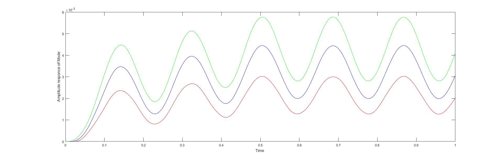
[y,t,x] = lsim(H,output_of_pice_func,time_sample);
plot(t,y(:,1),'r')
hold on
plot(t,y(:,2),'b')
plot(t,y(:,3),'g')
hold off
The responce looks like this
Email: [email protected]